dt <- data.frame(

 x1 = c(7,1,11,11,7,11,3,1,2,21,1,11,10),
 x2 = c(26,29,56,31,52,55,71,31,54,47,40,66,68),
 x3 = c(6,15,8,8,6,9,17,22,18,4,23,9,8),
 x4 = c(60,52,20,47,33,22,6,44,22,26,34,12,12),
 y = c(78.5,74.3,104.3,87.6,95.9,109.2,102.7,72.5,93.1,115.9,83.8,113.3,109.4)
)해당 자료는 전북대학교 이영미 교수님 2023응용통계학 자료임
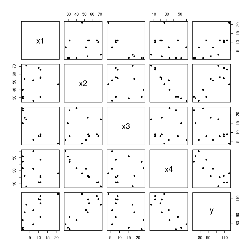
변수선택
pairs(dt, pch=16)
cor(dt)| x1 | x2 | x3 | x4 | y | |
|---|---|---|---|---|---|
| x1 | 1.0000000 | 0.2285795 | -0.8241338 | -0.2454451 | 0.7307175 |
| x2 | 0.2285795 | 1.0000000 | -0.1392424 | -0.9729550 | 0.8162526 |
| x3 | -0.8241338 | -0.1392424 | 1.0000000 | 0.0295370 | -0.5346707 |
| x4 | -0.2454451 | -0.9729550 | 0.0295370 | 1.0000000 | -0.8213050 |
| y | 0.7307175 | 0.8162526 | -0.5346707 | -0.8213050 | 1.0000000 |
- Full Model : \(𝑦 = 𝛽_0 + 𝛽_1𝑥_1 + 𝛽_2𝑥_2 + 𝛽_3𝑥_3 + 𝛽_4𝑥_4 + \epsilon\)
m <- lm(y~., dt) ##FM
summary(m)
Call:
lm(formula = y ~ ., data = dt)

Residuals:
    Min      1Q  Median      3Q     Max
-3.1750 -1.6709  0.2508  1.3783  3.9254

Coefficients:
            Estimate Std. Error t value Pr(>|t|)
(Intercept)  62.4054    70.0710   0.891   0.3991
x1            1.5511     0.7448   2.083   0.0708 .
x2            0.5102     0.7238   0.705   0.5009
x3            0.1019     0.7547   0.135   0.8959
x4           -0.1441     0.7091  -0.203   0.8441
---
Signif. codes:  0 ‘***’ 0.001 ‘**’ 0.01 ‘*’ 0.05 ‘.’ 0.1 ‘ ’ 1

Residual standard error: 2.446 on 8 degrees of freedom
Multiple R-squared:  0.9824,    Adjusted R-squared:  0.9736
F-statistic: 111.5 on 4 and 8 DF,  p-value: 4.756e-07
모형은 유의하게 나오고 R^2도 값이 크게나오는데, 회귀계수는 하나도 유의한게 없다? 다중공산성 때문에
후진제거법
summary(m)
Call:
lm(formula = y ~ ., data = dt)

Residuals:
    Min      1Q  Median      3Q     Max
-3.1750 -1.6709  0.2508  1.3783  3.9254

Coefficients:
            Estimate Std. Error t value Pr(>|t|)
(Intercept)  62.4054    70.0710   0.891   0.3991
x1            1.5511     0.7448   2.083   0.0708 .
x2            0.5102     0.7238   0.705   0.5009
x3            0.1019     0.7547   0.135   0.8959
x4           -0.1441     0.7091  -0.203   0.8441
---
Signif. codes:  0 ‘***’ 0.001 ‘**’ 0.01 ‘*’ 0.05 ‘.’ 0.1 ‘ ’ 1

Residual standard error: 2.446 on 8 degrees of freedom
Multiple R-squared:  0.9824,    Adjusted R-squared:  0.9736
F-statistic: 111.5 on 4 and 8 DF,  p-value: 4.756e-07
부분 F통계량, F통계량 = t^2 (t검정)
\(H_0:\beta_1= 0\)
위의
t value제곱하면 부분 F통계량이 됨t-value의 절대값이 가장 작은 값을 찾아주면 됨 -> x3
drop1(m, test = "F") #x3 제거
# m에서 F통계량 사요하여 제거한것 확인| Df | Sum of Sq | RSS | AIC | F value | Pr(>F) | |
|---|---|---|---|---|---|---|
| <dbl> | <dbl> | <dbl> | <dbl> | <dbl> | <dbl> | |
| <none> | NA | NA | 47.86364 | 26.94429 | NA | NA |
| x1 | 1 | 25.9509114 | 73.81455 | 30.57588 | 4.33747400 | 0.07082169 |
| x2 | 1 | 2.9724782 | 50.83612 | 25.72755 | 0.49682444 | 0.50090110 |
| x3 | 1 | 0.1090900 | 47.97273 | 24.97388 | 0.01823347 | 0.89592269 |
| x4 | 1 | 0.2469747 | 48.11061 | 25.01120 | 0.04127972 | 0.84407147 |
RSS: SSE
F value: \(F=\dfrac{SSE_{RM}-SSE_{FM}}{SSE_{FM}/(n-p-1)}\) F값이 작을수록 유의하지 않다. 클수록 유의하다.3번째값이 가장 작은 값을 갖다. 유의확률이 제일 크니까 변수가 제거된다.
m1 <- update(m, ~ . -x3)
summary(m1) #x4 제거
Call:
lm(formula = y ~ x1 + x2 + x4, data = dt)

Residuals:
    Min      1Q  Median      3Q     Max
-3.0919 -1.8016  0.2562  1.2818  3.8982

Coefficients:
            Estimate Std. Error t value Pr(>|t|)
(Intercept)  71.6483    14.1424   5.066 0.000675 ***
x1            1.4519     0.1170  12.410 5.78e-07 ***
x2            0.4161     0.1856   2.242 0.051687 .
x4           -0.2365     0.1733  -1.365 0.205395
---
Signif. codes:  0 ‘***’ 0.001 ‘**’ 0.01 ‘*’ 0.05 ‘.’ 0.1 ‘ ’ 1

Residual standard error: 2.309 on 9 degrees of freedom
Multiple R-squared:  0.9823,    Adjusted R-squared:  0.9764
F-statistic: 166.8 on 3 and 9 DF, p-value: 3.323e-08\(lm(y\)~\(x_1+x_2+x_4, dt)\) 라고 표현해도 된다.
x1이 유의해졌다. (x3과 다중공산성이 심했었다)
drop1(m1, test = "F")| Df | Sum of Sq | RSS | AIC | F value | Pr(>F) | |
|---|---|---|---|---|---|---|
| <dbl> | <dbl> | <dbl> | <dbl> | <dbl> | <dbl> | |
| <none> | NA | NA | 47.97273 | 24.97388 | NA | NA |
| x1 | 1 | 820.907402 | 868.88013 | 60.62933 | 154.007635 | 5.780764e-07 |
| x2 | 1 | 26.789383 | 74.76211 | 28.74170 | 5.025865 | 5.168735e-02 |
| x4 | 1 | 9.931754 | 57.90448 | 25.41999 | 1.863262 | 2.053954e-01 |
Fvalue의 x4가 가장 작으므로 제거하자. 유의하지 않다.
m2 <- update(m1, ~ . -x4)
summary(m2)
Call:
lm(formula = y ~ x1 + x2, data = dt)

Residuals:
   Min     1Q Median     3Q    Max
-2.893 -1.574 -1.302  1.363  4.048

Coefficients:
            Estimate Std. Error t value Pr(>|t|)
(Intercept) 52.57735    2.28617   23.00 5.46e-10 ***
x1           1.46831    0.12130   12.11 2.69e-07 ***
x2           0.66225    0.04585   14.44 5.03e-08 ***
---
Signif. codes:  0 ‘***’ 0.001 ‘**’ 0.01 ‘*’ 0.05 ‘.’ 0.1 ‘ ’ 1

Residual standard error: 2.406 on 10 degrees of freedom
Multiple R-squared:  0.9787,    Adjusted R-squared:  0.9744
F-statistic: 229.5 on 2 and 10 DF, p-value: 4.407e-09drop1(m2, test = "F")| Df | Sum of Sq | RSS | AIC | F value | Pr(>F) | |
|---|---|---|---|---|---|---|
| <dbl> | <dbl> | <dbl> | <dbl> | <dbl> | <dbl> | |
| <none> | NA | NA | 57.90448 | 25.41999 | NA | NA |
| x1 | 1 | 848.4319 | 906.33634 | 59.17799 | 146.5227 | 2.692212e-07 |
| x2 | 1 | 1207.7823 | 1265.68675 | 63.51947 | 208.5818 | 5.028960e-08 |
F value가 작은 x1을 제거할까? 하고 보니까 통계적으로 유의하므로 제거하지 않는다.
전진선택법
- Start model : \(𝑦 = 𝛽_0 + \epsilon\)
m0 = lm(y ~ 1, data = dt)add1(m0,
scope = y ~ x1 + x2 + x3+ x4,
test = "F") ## x4추가| Df | Sum of Sq | RSS | AIC | F value | Pr(>F) | |
|---|---|---|---|---|---|---|
| <dbl> | <dbl> | <dbl> | <dbl> | <dbl> | <dbl> | |
| <none> | NA | NA | 2715.7631 | 71.44443 | NA | NA |
| x1 | 1 | 1450.0763 | 1265.6867 | 63.51947 | 12.602518 | 0.0045520446 |
| x2 | 1 | 1809.4267 | 906.3363 | 59.17799 | 21.960605 | 0.0006648249 |
| x3 | 1 | 776.3626 | 1939.4005 | 69.06740 | 4.403417 | 0.0597623242 |
| x4 | 1 | 1831.8962 | 883.8669 | 58.85164 | 22.798520 | 0.0005762318 |
F값이 크면 좋음. x4가 좋으니까 보면 유의하므로 추가하자.
m1 <- update(m0, ~ . +x4)
summary(m1)
Call:
lm(formula = y ~ x4, data = dt)

Residuals:
    Min      1Q  Median      3Q     Max
-12.589  -8.228   1.495   4.726  17.524

Coefficients:
            Estimate Std. Error t value Pr(>|t|)
(Intercept) 117.5679     5.2622  22.342 1.62e-10 ***
x4           -0.7382     0.1546  -4.775 0.000576 ***
---
Signif. codes:  0 ‘***’ 0.001 ‘**’ 0.01 ‘*’ 0.05 ‘.’ 0.1 ‘ ’ 1

Residual standard error: 8.964 on 11 degrees of freedom
Multiple R-squared:  0.6745,    Adjusted R-squared:  0.645
F-statistic: 22.8 on 1 and 11 DF, p-value: 0.0005762add1(m1,
scope = y ~ x1 + x2 + x3+ x4,
test = "F") ## x1추가| Df | Sum of Sq | RSS | AIC | F value | Pr(>F) | |
|---|---|---|---|---|---|---|
| <dbl> | <dbl> | <dbl> | <dbl> | <dbl> | <dbl> | |
| <none> | NA | NA | 883.86692 | 58.85164 | NA | NA |
| x1 | 1 | 809.10480 | 74.76211 | 28.74170 | 108.2239093 | 1.105281e-06 |
| x2 | 1 | 14.98679 | 868.88013 | 60.62933 | 0.1724839 | 6.866842e-01 |
| x3 | 1 | 708.12891 | 175.73800 | 39.85258 | 40.2945802 | 8.375467e-05 |
x1의 F갑싱 제일 크고 유의하므로 추가
m2 <- update(m1, ~ . +x1)
summary(m2)
Call:
lm(formula = y ~ x4 + x1, data = dt)

Residuals:
    Min      1Q  Median      3Q     Max
-5.0234 -1.4737  0.1371  1.7305  3.7701

Coefficients:
             Estimate Std. Error t value Pr(>|t|)
(Intercept) 103.09738    2.12398   48.54 3.32e-13 ***
x4           -0.61395    0.04864  -12.62 1.81e-07 ***
x1            1.43996    0.13842   10.40 1.11e-06 ***
---
Signif. codes:  0 ‘***’ 0.001 ‘**’ 0.01 ‘*’ 0.05 ‘.’ 0.1 ‘ ’ 1

Residual standard error: 2.734 on 10 degrees of freedom
Multiple R-squared:  0.9725,    Adjusted R-squared:  0.967
F-statistic: 176.6 on 2 and 10 DF, p-value: 1.581e-08add1(m2,
scope = y ~ x1 + x2 + x3+ x4,
test = "F") ## stop| Df | Sum of Sq | RSS | AIC | F value | Pr(>F) | |
|---|---|---|---|---|---|---|
| <dbl> | <dbl> | <dbl> | <dbl> | <dbl> | <dbl> | |
| <none> | NA | NA | 74.76211 | 28.74170 | NA | NA |
| x2 | 1 | 26.78938 | 47.97273 | 24.97388 | 5.025865 | 0.05168735 |
| x3 | 1 | 23.92599 | 50.83612 | 25.72755 | 4.235846 | 0.06969226 |
x2의 F값이 더 크지만, pr값이 애매해. 유의수준 a=0.05면 유의하지 않다. 모형에 포함될 수 없으므로 멈춘다.
최종 모형은 x1과 x4를 선택한 모형
단계적선택법
m0 = lm(y ~ 1, data = dt)
# 절편먼저 시작add1(m0,
scope = y ~ x1 + x2 + x3+ x4,
test = "F") ## x4추가| Df | Sum of Sq | RSS | AIC | F value | Pr(>F) | |
|---|---|---|---|---|---|---|
| <dbl> | <dbl> | <dbl> | <dbl> | <dbl> | <dbl> | |
| <none> | NA | NA | 2715.7631 | 71.44443 | NA | NA |
| x1 | 1 | 1450.0763 | 1265.6867 | 63.51947 | 12.602518 | 0.0045520446 |
| x2 | 1 | 1809.4267 | 906.3363 | 59.17799 | 21.960605 | 0.0006648249 |
| x3 | 1 | 776.3626 | 1939.4005 | 69.06740 | 4.403417 | 0.0597623242 |
| x4 | 1 | 1831.8962 | 883.8669 | 58.85164 | 22.798520 | 0.0005762318 |
m1 <- update(m0, ~ . +x4)
summary(m1)
Call:
lm(formula = y ~ x4, data = dt)

Residuals:
    Min      1Q  Median      3Q     Max
-12.589  -8.228   1.495   4.726  17.524

Coefficients:
            Estimate Std. Error t value Pr(>|t|)
(Intercept) 117.5679     5.2622  22.342 1.62e-10 ***
x4           -0.7382     0.1546  -4.775 0.000576 ***
---
Signif. codes:  0 ‘***’ 0.001 ‘**’ 0.01 ‘*’ 0.05 ‘.’ 0.1 ‘ ’ 1

Residual standard error: 8.964 on 11 degrees of freedom
Multiple R-squared:  0.6745,    Adjusted R-squared:  0.645
F-statistic: 22.8 on 1 and 11 DF, p-value: 0.0005762add1(m1,
scope = y ~ x1 + x2 + x3+ x4,
test = "F") ## x1추가| Df | Sum of Sq | RSS | AIC | F value | Pr(>F) | |
|---|---|---|---|---|---|---|
| <dbl> | <dbl> | <dbl> | <dbl> | <dbl> | <dbl> | |
| <none> | NA | NA | 883.86692 | 58.85164 | NA | NA |
| x1 | 1 | 809.10480 | 74.76211 | 28.74170 | 108.2239093 | 1.105281e-06 |
| x2 | 1 | 14.98679 | 868.88013 | 60.62933 | 0.1724839 | 6.866842e-01 |
| x3 | 1 | 708.12891 | 175.73800 | 39.85258 | 40.2945802 | 8.375467e-05 |
m2 <- update(m1, ~ . +x1)drop1(m2, test = "F") #제거 없음| Df | Sum of Sq | RSS | AIC | F value | Pr(>F) | |
|---|---|---|---|---|---|---|
| <dbl> | <dbl> | <dbl> | <dbl> | <dbl> | <dbl> | |
| <none> | NA | NA | 74.76211 | 28.74170 | NA | NA |
| x4 | 1 | 1190.9246 | 1265.68675 | 63.51947 | 159.2952 | 1.814890e-07 |
| x1 | 1 | 809.1048 | 883.86692 | 58.85164 | 108.2239 | 1.105281e-06 |
x1,x4 유의하니까 그대로 가져가자
add1(m2,
 scope = y ~ x1 + x2 + x3+ x4,
test = "F") ## x2추가| Df | Sum of Sq | RSS | AIC | F value | Pr(>F) | |
|---|---|---|---|---|---|---|
| <dbl> | <dbl> | <dbl> | <dbl> | <dbl> | <dbl> | |
| <none> | NA | NA | 74.76211 | 28.74170 | NA | NA |
| x2 | 1 | 26.78938 | 47.97273 | 24.97388 | 5.025865 | 0.05168735 |
| x3 | 1 | 23.92599 | 50.83612 | 25.72755 | 4.235846 | 0.06969226 |
유의수준 a=0.1로 보자
m3 <- update(m2, ~ . +x2)
summary(m3)
Call:
lm(formula = y ~ x4 + x1 + x2, data = dt)

Residuals:
    Min      1Q  Median      3Q     Max
-3.0919 -1.8016  0.2562  1.2818  3.8982

Coefficients:
            Estimate Std. Error t value Pr(>|t|)
(Intercept)  71.6483    14.1424   5.066 0.000675 ***
x4           -0.2365     0.1733  -1.365 0.205395
x1            1.4519     0.1170  12.410 5.78e-07 ***
x2            0.4161     0.1856   2.242 0.051687 .
---
Signif. codes:  0 ‘***’ 0.001 ‘**’ 0.01 ‘*’ 0.05 ‘.’ 0.1 ‘ ’ 1

Residual standard error: 2.309 on 9 degrees of freedom
Multiple R-squared:  0.9823,    Adjusted R-squared:  0.9764
F-statistic: 166.8 on 3 and 9 DF, p-value: 3.323e-08drop1(m3, test="F") #x4 제거| Df | Sum of Sq | RSS | AIC | F value | Pr(>F) | |
|---|---|---|---|---|---|---|
| <dbl> | <dbl> | <dbl> | <dbl> | <dbl> | <dbl> | |
| <none> | NA | NA | 47.97273 | 24.97388 | NA | NA |
| x4 | 1 | 9.931754 | 57.90448 | 25.41999 | 1.863262 | 2.053954e-01 |
| x1 | 1 | 820.907402 | 868.88013 | 60.62933 | 154.007635 | 5.780764e-07 |
| x2 | 1 | 26.789383 | 74.76211 | 28.74170 | 5.025865 | 5.168735e-02 |
x2를 추가했기 때문에 x2는 보지 않고 x1과 x4만 보면 된다
m4 <- update(m3, ~ . -x4)
summary(m4)
Call:
lm(formula = y ~ x1 + x2, data = dt)

Residuals:
   Min     1Q Median     3Q    Max
-2.893 -1.574 -1.302  1.363  4.048

Coefficients:
            Estimate Std. Error t value Pr(>|t|)
(Intercept) 52.57735    2.28617   23.00 5.46e-10 ***
x1           1.46831    0.12130   12.11 2.69e-07 ***
x2           0.66225    0.04585   14.44 5.03e-08 ***
---
Signif. codes:  0 ‘***’ 0.001 ‘**’ 0.01 ‘*’ 0.05 ‘.’ 0.1 ‘ ’ 1

Residual standard error: 2.406 on 10 degrees of freedom
Multiple R-squared:  0.9787,    Adjusted R-squared:  0.9744
F-statistic: 229.5 on 2 and 10 DF, p-value: 4.407e-09add1(m4,
scope = y ~ x1 + x2 + x3+ x4,
test = "F") #stop| Df | Sum of Sq | RSS | AIC | F value | Pr(>F) | |
|---|---|---|---|---|---|---|
| <dbl> | <dbl> | <dbl> | <dbl> | <dbl> | <dbl> | |
| <none> | NA | NA | 57.90448 | 25.41999 | NA | NA |
| x3 | 1 | 9.793869 | 48.11061 | 25.01120 | 1.832128 | 0.2088895 |
| x4 | 1 | 9.931754 | 47.97273 | 24.97388 | 1.863262 | 0.2053954 |
AIC를 이용한 변수 선택법
- 모델 선택시 AIC가 작은 모델을 선택
Backward - AIC
후진제거법 AIC로 해보기
step 함수: AIC가 기준임
model_back = step(m, direction = "backward")
summary(model_back)
Start: AIC=26.94
y ~ x1 + x2 + x3 + x4
Df Sum of Sq RSS AIC
- x3 1 0.1091 47.973 24.974
- x4 1 0.2470 48.111 25.011
- x2 1 2.9725 50.836 25.728
<none> 47.864 26.944
- x1 1 25.9509 73.815 30.576
Step: AIC=24.97
y ~ x1 + x2 + x4
Df Sum of Sq RSS AIC
<none> 47.97 24.974
- x4 1 9.93 57.90 25.420
- x2 1 26.79 74.76 28.742
- x1 1 820.91 868.88 60.629
Call:
lm(formula = y ~ x1 + x2 + x4, data = dt)

Residuals:
    Min      1Q  Median      3Q     Max
-3.0919 -1.8016  0.2562  1.2818  3.8982

Coefficients:
            Estimate Std. Error t value Pr(>|t|)
(Intercept)  71.6483    14.1424   5.066 0.000675 ***
x1            1.4519     0.1170  12.410 5.78e-07 ***
x2            0.4161     0.1856   2.242 0.051687 .
x4           -0.2365     0.1733  -1.365 0.205395
---
Signif. codes:  0 ‘***’ 0.001 ‘**’ 0.01 ‘*’ 0.05 ‘.’ 0.1 ‘ ’ 1

Residual standard error: 2.309 on 9 degrees of freedom
Multiple R-squared:  0.9823,    Adjusted R-squared:  0.9764
F-statistic: 166.8 on 3 and 9 DF,  p-value: 3.323e-08
Df Sum of Sq RSS AIC
- x3 1 0.1091 47.973 24.974
- x4 1 0.2470 48.111 25.011
- x2 1 2.9725 50.836 25.728
<none> 47.864 26.944
- x1 1 25.9509 73.815 30.576-x3을 뺐을때 aic.. -x4을 뺏을때 aic…
AIC가 작으면 작을수록 좋다.그래서 x3빼자
x2와 x4가 애매하긴 하지만,,
Forward - AIC
- 전진선택법
model_forward = step(
 m0,
 scope = y ~ x1 + x2 + x3+ x4,
 direction = "forward")
summary(model_forward)
Start: AIC=71.44
y ~ 1
Df Sum of Sq RSS AIC
+ x4 1 1831.90 883.87 58.852
+ x2 1 1809.43 906.34 59.178
+ x1 1 1450.08 1265.69 63.519
+ x3 1 776.36 1939.40 69.067
<none> 2715.76 71.444
Step: AIC=58.85
y ~ x4
Df Sum of Sq RSS AIC
+ x1 1 809.10 74.76 28.742
+ x3 1 708.13 175.74 39.853
<none> 883.87 58.852
+ x2 1 14.99 868.88 60.629
Step: AIC=28.74
y ~ x4 + x1
Df Sum of Sq RSS AIC
+ x2 1 26.789 47.973 24.974
+ x3 1 23.926 50.836 25.728
<none> 74.762 28.742
Step: AIC=24.97
y ~ x4 + x1 + x2
Df Sum of Sq RSS AIC
<none> 47.973 24.974
+ x3 1 0.10909 47.864 26.944
Call:
lm(formula = y ~ x4 + x1 + x2, data = dt)

Residuals:
    Min      1Q  Median      3Q     Max
-3.0919 -1.8016  0.2562  1.2818  3.8982

Coefficients:
            Estimate Std. Error t value Pr(>|t|)
(Intercept)  71.6483    14.1424   5.066 0.000675 ***
x4           -0.2365     0.1733  -1.365 0.205395
x1            1.4519     0.1170  12.410 5.78e-07 ***
x2            0.4161     0.1856   2.242 0.051687 .
---
Signif. codes:  0 ‘***’ 0.001 ‘**’ 0.01 ‘*’ 0.05 ‘.’ 0.1 ‘ ’ 1

Residual standard error: 2.309 on 9 degrees of freedom
Multiple R-squared:  0.9823,    Adjusted R-squared:  0.9764
F-statistic: 166.8 on 3 and 9 DF,  p-value: 3.323e-08
Step - AIC
model_step = step(
 m0,
 scope = y ~ x1 + x2 + x3+ x4,
 direction = "both")
summary(model_step)
Start: AIC=71.44
y ~ 1
Df Sum of Sq RSS AIC
+ x4 1 1831.90 883.87 58.852
+ x2 1 1809.43 906.34 59.178
+ x1 1 1450.08 1265.69 63.519
+ x3 1 776.36 1939.40 69.067
<none> 2715.76 71.444
Step: AIC=58.85
y ~ x4
Df Sum of Sq RSS AIC
+ x1 1 809.10 74.76 28.742
+ x3 1 708.13 175.74 39.853
<none> 883.87 58.852
+ x2 1 14.99 868.88 60.629
- x4 1 1831.90 2715.76 71.444
Step: AIC=28.74
y ~ x4 + x1
Df Sum of Sq RSS AIC
+ x2 1 26.79 47.97 24.974
+ x3 1 23.93 50.84 25.728
<none> 74.76 28.742
- x1 1 809.10 883.87 58.852
- x4 1 1190.92 1265.69 63.519
Step: AIC=24.97
y ~ x4 + x1 + x2
Df Sum of Sq RSS AIC
<none> 47.97 24.974
- x4 1 9.93 57.90 25.420
+ x3 1 0.11 47.86 26.944
- x2 1 26.79 74.76 28.742
- x1 1 820.91 868.88 60.629
Call:
lm(formula = y ~ x4 + x1 + x2, data = dt)

Residuals:
    Min      1Q  Median      3Q     Max
-3.0919 -1.8016  0.2562  1.2818  3.8982

Coefficients:
            Estimate Std. Error t value Pr(>|t|)
(Intercept)  71.6483    14.1424   5.066 0.000675 ***
x4           -0.2365     0.1733  -1.365 0.205395
x1            1.4519     0.1170  12.410 5.78e-07 ***
x2            0.4161     0.1856   2.242 0.051687 .
---
Signif. codes:  0 ‘***’ 0.001 ‘**’ 0.01 ‘*’ 0.05 ‘.’ 0.1 ‘ ’ 1

Residual standard error: 2.309 on 9 degrees of freedom
Multiple R-squared:  0.9823,    Adjusted R-squared:  0.9764
F-statistic: 166.8 on 3 and 9 DF, p-value: 3.323e-08- 추가하는거랑 빼는거랑 동시에 진행
regsubsets
m_full <-lm(y~.,dt)
summary(m_full)
Call:
lm(formula = y ~ ., data = dt)

Residuals:
    Min      1Q  Median      3Q     Max
-3.1750 -1.6709  0.2508  1.3783  3.9254

Coefficients:
            Estimate Std. Error t value Pr(>|t|)
(Intercept)  62.4054    70.0710   0.891   0.3991
x1            1.5511     0.7448   2.083   0.0708 .
x2            0.5102     0.7238   0.705   0.5009
x3            0.1019     0.7547   0.135   0.8959
x4           -0.1441     0.7091  -0.203   0.8441
---
Signif. codes:  0 ‘***’ 0.001 ‘**’ 0.01 ‘*’ 0.05 ‘.’ 0.1 ‘ ’ 1

Residual standard error: 2.446 on 8 degrees of freedom
Multiple R-squared:  0.9824,    Adjusted R-squared:  0.9736
F-statistic: 111.5 on 4 and 8 DF,  p-value: 4.756e-07
nbest=1
fit <- regsubsets(y~., data=dt, nbest=1, nvmax=9, method='exhaustive',)summary(fit)Subset selection object
Call: regsubsets.formula(y ~ ., data = dt, nbest = 1, nvmax = 9, method = "exhaustive",
)
4 Variables (and intercept)
Forced in Forced out
x1 FALSE FALSE
x2 FALSE FALSE
x3 FALSE FALSE
x4 FALSE FALSE
1 subsets of each size up to 4
Selection Algorithm: exhaustive
x1 x2 x3 x4
1 ( 1 ) " " " " " " "*"
2 ( 1 ) "*" "*" " " " "
3 ( 1 ) "*" "*" " " "*"
4 ( 1 ) "*" "*" "*" "*"- 설명변수 1개, 2개, 3개 , 4개썼을때 제일 좋은 모형을 불러와 :nbest=1
with(summary(fit), round(cbind(which,rss,rsq,adjr2,cp,bic),3))| (Intercept) | x1 | x2 | x3 | x4 | rss | rsq | adjr2 | cp | bic | |
|---|---|---|---|---|---|---|---|---|---|---|
| 1 | 1 | 0 | 0 | 0 | 1 | 883.867 | 0.675 | 0.645 | 138.731 | -9.463 |
| 2 | 1 | 1 | 1 | 0 | 0 | 57.904 | 0.979 | 0.974 | 2.678 | -42.330 |
| 3 | 1 | 1 | 1 | 0 | 1 | 47.973 | 0.982 | 0.976 | 3.018 | -42.211 |
| 4 | 1 | 1 | 1 | 1 | 1 | 47.864 | 0.982 | 0.974 | 5.000 | -39.675 |
nbest=2
fit <- regsubsets(y~., data=dt, nbest=2, nvmax=9, method='exhaustive',)summary(fit)Subset selection object
Call: regsubsets.formula(y ~ ., data = dt, nbest = 2, nvmax = 9, method = "exhaustive",
)
4 Variables (and intercept)
Forced in Forced out
x1 FALSE FALSE
x2 FALSE FALSE
x3 FALSE FALSE
x4 FALSE FALSE
2 subsets of each size up to 4
Selection Algorithm: exhaustive
x1 x2 x3 x4
1 ( 1 ) " " " " " " "*"
1 ( 2 ) " " "*" " " " "
2 ( 1 ) "*" "*" " " " "
2 ( 2 ) "*" " " " " "*"
3 ( 1 ) "*" "*" " " "*"
3 ( 2 ) "*" "*" "*" " "
4 ( 1 ) "*" "*" "*" "*"- 좋았던걸 2개씩 리턴
nbest=6
fit <- regsubsets(y~., data=dt, nbest=6, nvmax=9, method='exhaustive',)
summary(fit)
Subset selection object
Call: regsubsets.formula(y ~ ., data = dt, nbest = 6, nvmax = 9, method = "exhaustive",
)
4 Variables (and intercept)
Forced in Forced out
x1 FALSE FALSE
x2 FALSE FALSE
x3 FALSE FALSE
x4 FALSE FALSE
6 subsets of each size up to 4
Selection Algorithm: exhaustive
x1 x2 x3 x4
1 ( 1 ) " " " " " " "*"
1 ( 2 ) " " "*" " " " "
1 ( 3 ) "*" " " " " " "
1 ( 4 ) " " " " "*" " "
2 ( 1 ) "*" "*" " " " "
2 ( 2 ) "*" " " " " "*"
2 ( 3 ) " " " " "*" "*"
2 ( 4 ) " " "*" "*" " "
2 ( 5 ) " " "*" " " "*"
2 ( 6 ) "*" " " "*" " "
3 ( 1 ) "*" "*" " " "*"
3 ( 2 ) "*" "*" "*" " "
3 ( 3 ) "*" " " "*" "*"
3 ( 4 ) " " "*" "*" "*"
4 ( 1 ) "*" "*" "*" "*"with(summary(fit), round(cbind(which,rss,rsq,adjr2,cp,bic),3))| (Intercept) | x1 | x2 | x3 | x4 | rss | rsq | adjr2 | cp | bic | |
|---|---|---|---|---|---|---|---|---|---|---|
| 1 | 1 | 0 | 0 | 0 | 1 | 883.867 | 0.675 | 0.645 | 138.731 | -9.463 |
| 1 | 1 | 0 | 1 | 0 | 0 | 906.336 | 0.666 | 0.636 | 142.486 | -9.137 |
| 1 | 1 | 1 | 0 | 0 | 0 | 1265.687 | 0.534 | 0.492 | 202.549 | -4.795 |
| 1 | 1 | 0 | 0 | 1 | 0 | 1939.400 | 0.286 | 0.221 | 315.154 | 0.753 |
| 2 | 1 | 1 | 1 | 0 | 0 | 57.904 | 0.979 | 0.974 | 2.678 | -42.330 |
| 2 | 1 | 1 | 0 | 0 | 1 | 74.762 | 0.972 | 0.967 | 5.496 | -39.008 |
| 2 | 1 | 0 | 0 | 1 | 1 | 175.738 | 0.935 | 0.922 | 22.373 | -27.897 |
| 2 | 1 | 0 | 1 | 1 | 0 | 415.443 | 0.847 | 0.816 | 62.438 | -16.712 |
| 2 | 1 | 0 | 1 | 0 | 1 | 868.880 | 0.680 | 0.616 | 138.226 | -7.120 |
| 2 | 1 | 1 | 0 | 1 | 0 | 1227.072 | 0.548 | 0.458 | 198.095 | -2.633 |
| 3 | 1 | 1 | 1 | 0 | 1 | 47.973 | 0.982 | 0.976 | 3.018 | -42.211 |
| 3 | 1 | 1 | 1 | 1 | 0 | 48.111 | 0.982 | 0.976 | 3.041 | -42.173 |
| 3 | 1 | 1 | 0 | 1 | 1 | 50.836 | 0.981 | 0.975 | 3.497 | -41.457 |
| 3 | 1 | 0 | 1 | 1 | 1 | 73.815 | 0.973 | 0.964 | 7.337 | -36.609 |
| 4 | 1 | 1 | 1 | 1 | 1 | 47.864 | 0.982 | 0.974 | 5.000 | -39.675 |
nvmax=2
- 설명변수 최대 2개까지만
fit <- regsubsets(y~., data=dt, nbest=6, nvmax=2, method='exhaustive',)
summary(fit)
Subset selection object
Call: regsubsets.formula(y ~ ., data = dt, nbest = 6, nvmax = 2, method = "exhaustive",
)
4 Variables (and intercept)
Forced in Forced out
x1 FALSE FALSE
x2 FALSE FALSE
x3 FALSE FALSE
x4 FALSE FALSE
6 subsets of each size up to 2
Selection Algorithm: exhaustive
x1 x2 x3 x4
1 ( 1 ) " " " " " " "*"
1 ( 2 ) " " "*" " " " "
1 ( 3 ) "*" " " " " " "
1 ( 4 ) " " " " "*" " "
2 ( 1 ) "*" "*" " " " "
2 ( 2 ) "*" " " " " "*"
2 ( 3 ) " " " " "*" "*"
2 ( 4 ) " " "*" "*" " "
2 ( 5 ) " " "*" " " "*"
2 ( 6 ) "*" " " "*" " "자동차 연비 자료 분석
str(mtcars)'data.frame': 32 obs. of 11 variables:
$ mpg : num 21 21 22.8 21.4 18.7 18.1 14.3 24.4 22.8 19.2 ...
$ cyl : num 6 6 4 6 8 6 8 4 4 6 ...
$ disp: num 160 160 108 258 360 ...
$ hp : num 110 110 93 110 175 105 245 62 95 123 ...
$ drat: num 3.9 3.9 3.85 3.08 3.15 2.76 3.21 3.69 3.92 3.92 ...
$ wt : num 2.62 2.88 2.32 3.21 3.44 ...
$ qsec: num 16.5 17 18.6 19.4 17 ...
$ vs : num 0 0 1 1 0 1 0 1 1 1 ...
$ am : num 1 1 1 0 0 0 0 0 0 0 ...
$ gear: num 4 4 4 3 3 3 3 4 4 4 ...
$ carb: num 4 4 1 1 2 1 4 2 2 4 ...round(cor(mtcars),2)| mpg | cyl | disp | hp | drat | wt | qsec | vs | am | gear | carb | |
|---|---|---|---|---|---|---|---|---|---|---|---|
| mpg | 1.00 | -0.85 | -0.85 | -0.78 | 0.68 | -0.87 | 0.42 | 0.66 | 0.60 | 0.48 | -0.55 |
| cyl | -0.85 | 1.00 | 0.90 | 0.83 | -0.70 | 0.78 | -0.59 | -0.81 | -0.52 | -0.49 | 0.53 |
| disp | -0.85 | 0.90 | 1.00 | 0.79 | -0.71 | 0.89 | -0.43 | -0.71 | -0.59 | -0.56 | 0.39 |
| hp | -0.78 | 0.83 | 0.79 | 1.00 | -0.45 | 0.66 | -0.71 | -0.72 | -0.24 | -0.13 | 0.75 |
| drat | 0.68 | -0.70 | -0.71 | -0.45 | 1.00 | -0.71 | 0.09 | 0.44 | 0.71 | 0.70 | -0.09 |
| wt | -0.87 | 0.78 | 0.89 | 0.66 | -0.71 | 1.00 | -0.17 | -0.55 | -0.69 | -0.58 | 0.43 |
| qsec | 0.42 | -0.59 | -0.43 | -0.71 | 0.09 | -0.17 | 1.00 | 0.74 | -0.23 | -0.21 | -0.66 |
| vs | 0.66 | -0.81 | -0.71 | -0.72 | 0.44 | -0.55 | 0.74 | 1.00 | 0.17 | 0.21 | -0.57 |
| am | 0.60 | -0.52 | -0.59 | -0.24 | 0.71 | -0.69 | -0.23 | 0.17 | 1.00 | 0.79 | 0.06 |
| gear | 0.48 | -0.49 | -0.56 | -0.13 | 0.70 | -0.58 | -0.21 | 0.21 | 0.79 | 1.00 | 0.27 |
| carb | -0.55 | 0.53 | 0.39 | 0.75 | -0.09 | 0.43 | -0.66 | -0.57 | 0.06 | 0.27 | 1.00 |
mpg(연비)가 y이고 y와 상관관계가 가장 높은것은 wt(차무게), hp(마력)
m_full <- lm(mpg~., mtcars)
summary(m_full)
Call:
lm(formula = mpg ~ ., data = mtcars)

Residuals:
    Min      1Q  Median      3Q     Max
-3.4506 -1.6044 -0.1196  1.2193  4.6271

Coefficients:
            Estimate Std. Error t value Pr(>|t|)
(Intercept) 12.30337   18.71788   0.657   0.5181
cyl         -0.11144    1.04502  -0.107   0.9161
disp         0.01334    0.01786   0.747   0.4635
hp          -0.02148    0.02177  -0.987   0.3350
drat         0.78711    1.63537   0.481   0.6353
wt          -3.71530    1.89441  -1.961   0.0633 .
qsec         0.82104    0.73084   1.123   0.2739
vs           0.31776    2.10451   0.151   0.8814
am           2.52023    2.05665   1.225   0.2340
gear         0.65541    1.49326   0.439   0.6652
carb        -0.19942    0.82875  -0.241   0.8122
---
Signif. codes:  0 ‘***’ 0.001 ‘**’ 0.01 ‘*’ 0.05 ‘.’ 0.1 ‘ ’ 1

Residual standard error: 2.65 on 21 degrees of freedom
Multiple R-squared:  0.869, Adjusted R-squared:  0.8066
F-statistic: 13.93 on 10 and 21 DF,  p-value: 3.793e-07
다중공산성 떄문에 회귀계수는 다 유의하지 않게 나옴
library(leaps)fit<-regsubsets(mpg~., data=mtcars, nbest=1,nvmax=9,
# method=c("exhaustive"(모든가능한),"backward", "forward", "seqrep")
method='exhaustive',
)summary(fit)Subset selection object
Call: regsubsets.formula(mpg ~ ., data = mtcars, nbest = 1, nvmax = 9,
method = "exhaustive", )
10 Variables (and intercept)
Forced in Forced out
cyl FALSE FALSE
disp FALSE FALSE
hp FALSE FALSE
drat FALSE FALSE
wt FALSE FALSE
qsec FALSE FALSE
vs FALSE FALSE
am FALSE FALSE
gear FALSE FALSE
carb FALSE FALSE
1 subsets of each size up to 9
Selection Algorithm: exhaustive
cyl disp hp drat wt qsec vs am gear carb
1 ( 1 ) " " " " " " " " "*" " " " " " " " " " "
2 ( 1 ) "*" " " " " " " "*" " " " " " " " " " "
3 ( 1 ) " " " " " " " " "*" "*" " " "*" " " " "
4 ( 1 ) " " " " "*" " " "*" "*" " " "*" " " " "
5 ( 1 ) " " "*" "*" " " "*" "*" " " "*" " " " "
6 ( 1 ) " " "*" "*" "*" "*" "*" " " "*" " " " "
7 ( 1 ) " " "*" "*" "*" "*" "*" " " "*" "*" " "
8 ( 1 ) " " "*" "*" "*" "*" "*" " " "*" "*" "*"
9 ( 1 ) " " "*" "*" "*" "*" "*" "*" "*" "*" "*" 설명변수 2개를 쓴거는 \(_{10}C_{2}=45\)개 모형을 만들 수 있음. \(R^2\)을 봐서 좋은걸 보면 cyl이랑 wt쓴게 제일 좋은 모형이야.
설명변수 1개를 쓴다면 그 중에서 wt쓴거의 \(R^2\)가 제일 좋아.
설명변수 3개는 wt,qsec,am 쓴게 제일 좋아
Forced in: 나는 이 변수가 꼭 들어갔으면 좋겠어Forced out: 나는 이변수가 꼭 뺐으면 좋겠어10개 쓴거가 full model 이고 설명변수를 1개 2개 3개 쓴…
with(summary(fit),
round(cbind(which,rss,rsq,adjr2,cp,bic),3))| (Intercept) | cyl | disp | hp | drat | wt | qsec | vs | am | gear | carb | rss | rsq | adjr2 | cp | bic | |
|---|---|---|---|---|---|---|---|---|---|---|---|---|---|---|---|---|
| 1 | 1 | 0 | 0 | 0 | 0 | 1 | 0 | 0 | 0 | 0 | 0 | 278.322 | 0.753 | 0.745 | 11.627 | -37.795 |
| 2 | 1 | 1 | 0 | 0 | 0 | 1 | 0 | 0 | 0 | 0 | 0 | 191.172 | 0.830 | 0.819 | 1.219 | -46.348 |
| 3 | 1 | 0 | 0 | 0 | 0 | 1 | 1 | 0 | 1 | 0 | 0 | 169.286 | 0.850 | 0.834 | 0.103 | -46.773 |
| 4 | 1 | 0 | 0 | 1 | 0 | 1 | 1 | 0 | 1 | 0 | 0 | 160.066 | 0.858 | 0.837 | 0.790 | -45.099 |
| 5 | 1 | 0 | 1 | 1 | 0 | 1 | 1 | 0 | 1 | 0 | 0 | 153.438 | 0.864 | 0.838 | 1.846 | -42.987 |
| 6 | 1 | 0 | 1 | 1 | 1 | 1 | 1 | 0 | 1 | 0 | 0 | 150.093 | 0.867 | 0.835 | 3.370 | -40.227 |
| 7 | 1 | 0 | 1 | 1 | 1 | 1 | 1 | 0 | 1 | 1 | 0 | 148.528 | 0.868 | 0.830 | 5.147 | -37.096 |
| 8 | 1 | 0 | 1 | 1 | 1 | 1 | 1 | 0 | 1 | 1 | 1 | 147.843 | 0.869 | 0.823 | 7.050 | -33.779 |
| 9 | 1 | 0 | 1 | 1 | 1 | 1 | 1 | 1 | 1 | 1 | 1 | 147.574 | 0.869 | 0.815 | 9.011 | -30.371 |
which,rss,rsq,adjr2,cp,bic
which:어떤 변수를 썼는지?
rss: sse 작을 수록 좋다. ->
147.574제일작은데, 원래 제일 복잡한 모형이 제일 작다. 감소하는 차이를 보자..rsq : \(R^2\) 크면 좋은데 둔화되는 점까지 보자.
adjr2 : \(R^2_{adj}\) 크면 좋다.
0.8385개cp: 작으면 좋다. \(cp \leq p+1\)
0.1033개bic: 작으면 좋다.
-46.7733개
3개를 쓰는게 좋을 거 같다.
fit_3<-lm(mpg~wt+qsec+am,mtcars)
summary(fit_3)
Call:
lm(formula = mpg ~ wt + qsec + am, data = mtcars)

Residuals:
    Min      1Q  Median      3Q     Max
-3.4811 -1.5555 -0.7257  1.4110  4.6610

Coefficients:
            Estimate Std. Error t value Pr(>|t|)
(Intercept)   9.6178     6.9596   1.382 0.177915
wt           -3.9165     0.7112  -5.507 6.95e-06 ***
qsec          1.2259     0.2887   4.247 0.000216 ***
am            2.9358     1.4109   2.081 0.046716 *
---
Signif. codes:  0 ‘***’ 0.001 ‘**’ 0.01 ‘*’ 0.05 ‘.’ 0.1 ‘ ’ 1

Residual standard error: 2.459 on 28 degrees of freedom
Multiple R-squared:  0.8497,    Adjusted R-squared:  0.8336
F-statistic: 52.75 on 3 and 28 DF, p-value: 1.21e-11fit_4<-lm(mpg~hp+wt+qsec+am,mtcars)
summary(fit_4)
Call:
lm(formula = mpg ~ hp + wt + qsec + am, data = mtcars)

Residuals:
    Min      1Q  Median      3Q     Max
-3.4975 -1.5902 -0.1122  1.1795  4.5404

Coefficients:
            Estimate Std. Error t value Pr(>|t|)
(Intercept) 17.44019    9.31887   1.871  0.07215 .
hp          -0.01765    0.01415  -1.247  0.22309
wt          -3.23810    0.88990  -3.639  0.00114 **
qsec         0.81060    0.43887   1.847  0.07573 .
am           2.92550    1.39715   2.094  0.04579 *
---
Signif. codes:  0 ‘***’ 0.001 ‘**’ 0.01 ‘*’ 0.05 ‘.’ 0.1 ‘ ’ 1

Residual standard error: 2.435 on 27 degrees of freedom
Multiple R-squared:  0.8579,    Adjusted R-squared:  0.8368
F-statistic: 40.74 on 4 and 27 DF, p-value: 4.589e-11fit<-regsubsets(mpg~., data=mtcars, nbest=1,nvmax=9,
# method=c("exhaustive"(모든가능한),"backward", "forward", "seqrep")
method='backward',
)
summary(fit)Subset selection object
Call: regsubsets.formula(mpg ~ ., data = mtcars, nbest = 1, nvmax = 9,
method = "backward", )
10 Variables (and intercept)
Forced in Forced out
cyl FALSE FALSE
disp FALSE FALSE
hp FALSE FALSE
drat FALSE FALSE
wt FALSE FALSE
qsec FALSE FALSE
vs FALSE FALSE
am FALSE FALSE
gear FALSE FALSE
carb FALSE FALSE
1 subsets of each size up to 9
Selection Algorithm: backward
cyl disp hp drat wt qsec vs am gear carb
1 ( 1 ) " " " " " " " " "*" " " " " " " " " " "
2 ( 1 ) " " " " " " " " "*" "*" " " " " " " " "
3 ( 1 ) " " " " " " " " "*" "*" " " "*" " " " "
4 ( 1 ) " " " " "*" " " "*" "*" " " "*" " " " "
5 ( 1 ) " " "*" "*" " " "*" "*" " " "*" " " " "
6 ( 1 ) " " "*" "*" "*" "*" "*" " " "*" " " " "
7 ( 1 ) " " "*" "*" "*" "*" "*" " " "*" "*" " "
8 ( 1 ) " " "*" "*" "*" "*" "*" " " "*" "*" "*"
9 ( 1 ) " " "*" "*" "*" "*" "*" "*" "*" "*" "*" 10번째부터 시작해서 거꾸로 올라감. 맨처음에 cyl이 빠지고 9개
그다음 vs가 빠짐
그다음 carb가 빠짐.
fit<-regsubsets(mpg~., data=mtcars, nbest=45,nvmax=9,
method='exhaustive',
)
summary(fit)
ERROR: Error in leaps.exhaustive(a, really.big): Exhaustive search will be S L O W, must specify really.big=T- nbest값을 너무 크게 주면 값이 너무 많아져서 에러메시지가뜬다.
fit<-regsubsets(mpg~., data=mtcars, nbest=45,nvmax=9,
method='exhaustive', really.big=T
)
summary(fit)
Subset selection object
Call: regsubsets.formula(mpg ~ ., data = mtcars, nbest = 45, nvmax = 9,
method = "exhaustive", really.big = T)
10 Variables (and intercept)
Forced in Forced out
cyl FALSE FALSE
disp FALSE FALSE
hp FALSE FALSE
drat FALSE FALSE
wt FALSE FALSE
qsec FALSE FALSE
vs FALSE FALSE
am FALSE FALSE
gear FALSE FALSE
carb FALSE FALSE
45 subsets of each size up to 9
Selection Algorithm: exhaustive
cyl disp hp drat wt qsec vs am gear carb
1 ( 1 ) " " " " " " " " "*" " " " " " " " " " "
1 ( 2 ) "*" " " " " " " " " " " " " " " " " " "
1 ( 3 ) " " "*" " " " " " " " " " " " " " " " "
1 ( 4 ) " " " " "*" " " " " " " " " " " " " " "
1 ( 5 ) " " " " " " "*" " " " " " " " " " " " "
1 ( 6 ) " " " " " " " " " " " " "*" " " " " " "
1 ( 7 ) " " " " " " " " " " " " " " "*" " " " "
1 ( 8 ) " " " " " " " " " " " " " " " " " " "*"
1 ( 9 ) " " " " " " " " " " " " " " " " "*" " "
1 ( 10 ) " " " " " " " " " " "*" " " " " " " " "
2 ( 1 ) "*" " " " " " " "*" " " " " " " " " " "
2 ( 2 ) " " " " "*" " " "*" " " " " " " " " " "
2 ( 3 ) " " " " " " " " "*" "*" " " " " " " " "
2 ( 4 ) " " " " " " " " "*" " " "*" " " " " " "
2 ( 5 ) " " " " " " " " "*" " " " " " " " " "*"
2 ( 6 ) " " " " "*" " " " " " " " " "*" " " " "
2 ( 7 ) " " "*" " " " " "*" " " " " " " " " " "
2 ( 8 ) " " "*" " " " " " " " " " " " " " " "*"
2 ( 9 ) " " " " " " "*" "*" " " " " " " " " " "
2 ( 10 ) "*" "*" " " " " " " " " " " " " " " " "
2 ( 11 ) "*" " " " " " " " " " " " " "*" " " " "
2 ( 12 ) " " " " " " " " "*" " " " " " " "*" " "
2 ( 13 ) " " " " " " " " "*" " " " " "*" " " " "
2 ( 14 ) " " " " "*" " " " " " " " " " " "*" " "
2 ( 15 ) " " "*" "*" " " " " " " " " " " " " " "
2 ( 16 ) " " " " "*" "*" " " " " " " " " " " " "
2 ( 17 ) "*" " " "*" " " " " " " " " " " " " " "
2 ( 18 ) "*" " " " " " " " " " " " " " " " " "*"
2 ( 19 ) "*" " " " " "*" " " " " " " " " " " " "
2 ( 20 ) "*" " " " " " " " " "*" " " " " " " " "
2 ( 21 ) " " " " " " " " " " " " " " " " "*" "*"
2 ( 22 ) " " "*" " " " " " " " " " " "*" " " " "
2 ( 23 ) " " "*" " " "*" " " " " " " " " " " " "
2 ( 24 ) "*" " " " " " " " " " " " " " " "*" " "
2 ( 25 ) "*" " " " " " " " " " " "*" " " " " " "
2 ( 26 ) " " "*" " " " " " " " " "*" " " " " " "
2 ( 27 ) " " "*" " " " " " " "*" " " " " " " " "
2 ( 28 ) " " "*" " " " " " " " " " " " " "*" " "
2 ( 29 ) " " " " " " "*" " " " " " " " " " " "*"
2 ( 30 ) " " " " " " " " " " " " " " "*" " " "*"
2 ( 31 ) " " " " " " " " " " "*" " " "*" " " " "
2 ( 32 ) " " " " " " " " " " " " "*" "*" " " " "
2 ( 33 ) " " " " "*" " " " " "*" " " " " " " " "
2 ( 34 ) " " " " " " "*" " " " " "*" " " " " " "
2 ( 35 ) " " " " "*" " " " " " " "*" " " " " " "
2 ( 36 ) " " " " "*" " " " " " " " " " " " " "*"
2 ( 37 ) " " " " " " "*" " " "*" " " " " " " " "
2 ( 38 ) " " " " " " " " " " " " "*" " " "*" " "
2 ( 39 ) " " " " " " " " " " "*" " " " " "*" " "
2 ( 40 ) " " " " " " "*" " " " " " " "*" " " " "
2 ( 41 ) " " " " " " " " " " " " "*" " " " " "*"
2 ( 42 ) " " " " " " "*" " " " " " " " " "*" " "
2 ( 43 ) " " " " " " " " " " "*" "*" " " " " " "
2 ( 44 ) " " " " " " " " " " " " " " "*" "*" " "
2 ( 45 ) " " " " " " " " " " "*" " " " " " " "*"
3 ( 1 ) " " " " " " " " "*" "*" " " "*" " " " "
3 ( 2 ) "*" " " "*" " " "*" " " " " " " " " " "
3 ( 3 ) "*" " " " " " " "*" " " " " " " " " "*"
3 ( 4 ) " " " " "*" " " "*" " " " " "*" " " " "
3 ( 5 ) "*" " " " " " " "*" "*" " " " " " " " "
3 ( 6 ) " " " " " " "*" "*" "*" " " " " " " " "
3 ( 7 ) " " " " "*" "*" "*" " " " " " " " " " "
3 ( 8 ) " " " " "*" " " "*" " " " " " " "*" " "
3 ( 9 ) " " " " "*" " " "*" "*" " " " " " " " "
3 ( 10 ) " " " " " " " " "*" "*" " " " " "*" " "
3 ( 11 ) "*" " " " " " " "*" " " " " " " "*" " "
3 ( 12 ) " " " " "*" " " "*" " " "*" " " " " " "
3 ( 13 ) "*" "*" " " " " "*" " " " " " " " " " "
3 ( 14 ) "*" " " " " " " "*" " " "*" " " " " " "
3 ( 15 ) "*" " " " " " " "*" " " " " "*" " " " "
3 ( 16 ) "*" " " " " "*" "*" " " " " " " " " " "
3 ( 17 ) " " "*" " " " " " " " " " " "*" " " "*"
3 ( 18 ) " " " " " " " " "*" "*" " " " " " " "*"
3 ( 19 ) " " " " "*" " " "*" " " " " " " " " "*"
3 ( 20 ) " " "*" "*" " " "*" " " " " " " " " " "
3 ( 21 ) " " " " " " " " "*" "*" "*" " " " " " "
3 ( 22 ) " " "*" " " " " "*" "*" " " " " " " " "
3 ( 23 ) " " " " " " "*" "*" " " " " " " " " "*"
3 ( 24 ) " " "*" " " " " " " " " " " " " "*" "*"
3 ( 25 ) " " "*" " " " " "*" " " " " " " " " "*"
3 ( 26 ) " " " " " " " " "*" " " " " " " "*" "*"
3 ( 27 ) " " " " " " " " "*" " " "*" " " " " "*"
3 ( 28 ) "*" " " " " " " " " " " " " "*" " " "*"
3 ( 29 ) " " "*" " " "*" " " " " " " " " " " "*"
3 ( 30 ) " " " " " " " " "*" " " " " "*" " " "*"
3 ( 31 ) " " " " " " " " "*" " " "*" "*" " " " "
3 ( 32 ) " " " " " " "*" "*" " " "*" " " " " " "
3 ( 33 ) " " " " "*" " " " " " " "*" "*" " " " "
3 ( 34 ) "*" " " "*" " " " " " " " " "*" " " " "
3 ( 35 ) " " "*" " " " " "*" " " "*" " " " " " "
3 ( 36 ) " " " " " " " " "*" " " "*" " " "*" " "
3 ( 37 ) " " "*" "*" " " " " " " " " "*" " " " "
3 ( 38 ) " " " " "*" " " " " " " " " "*" " " "*"
3 ( 39 ) " " " " "*" "*" " " " " " " "*" " " " "
3 ( 40 ) " " " " "*" " " " " " " " " " " "*" "*"
3 ( 41 ) "*" " " " " " " " " " " " " " " "*" "*"
3 ( 42 ) " " " " "*" " " " " " " " " "*" "*" " "
3 ( 43 ) " " " " "*" " " " " "*" " " "*" " " " "
3 ( 44 ) "*" "*" " " " " " " " " " " " " " " "*"
3 ( 45 ) " " "*" " " " " " " "*" " " " " " " "*"
4 ( 1 ) " " " " "*" " " "*" "*" " " "*" " " " "
4 ( 2 ) " " " " " " " " "*" "*" " " "*" " " "*"
4 ( 3 ) " " "*" " " " " "*" "*" " " "*" " " " "
4 ( 4 ) "*" " " " " " " "*" "*" " " "*" " " " "
4 ( 5 ) " " " " " " "*" "*" "*" " " "*" " " " "
4 ( 6 ) "*" " " " " " " "*" " " " " "*" " " "*"
4 ( 7 ) " " " " "*" " " "*" " " "*" "*" " " " "
4 ( 8 ) " " " " " " " " "*" "*" " " "*" "*" " "
4 ( 9 ) " " " " " " " " "*" "*" "*" "*" " " " "
4 ( 10 ) "*" " " "*" " " "*" " " " " "*" " " " "
4 ( 11 ) "*" "*" "*" " " "*" " " " " " " " " " "
4 ( 12 ) "*" " " " " "*" "*" " " " " " " " " "*"
4 ( 13 ) "*" " " " " " " "*" " " " " " " "*" "*"
4 ( 14 ) "*" " " "*" " " "*" " " " " " " " " "*"
4 ( 15 ) " " " " "*" "*" "*" "*" " " " " " " " "
4 ( 16 ) "*" " " "*" "*" "*" " " " " " " " " " "
4 ( 17 ) " " " " "*" " " "*" "*" " " " " "*" " "
4 ( 18 ) " " " " " " " " "*" "*" " " " " "*" "*"
4 ( 19 ) " " " " "*" " " "*" " " " " " " "*" "*"
4 ( 20 ) " " " " "*" " " "*" " " " " "*" " " "*"
4 ( 21 ) "*" " " "*" " " "*" "*" " " " " " " " "
4 ( 22 ) "*" "*" " " " " "*" "*" " " " " " " " "
4 ( 23 ) "*" " " "*" " " "*" " " " " " " "*" " "
4 ( 24 ) "*" " " " " " " "*" "*" " " " " " " "*"
4 ( 25 ) "*" " " "*" " " "*" " " "*" " " " " " "
4 ( 26 ) " " " " " " "*" "*" "*" " " " " " " "*"
4 ( 27 ) " " " " "*" "*" "*" " " " " "*" " " " "
4 ( 28 ) "*" "*" " " " " "*" " " " " " " " " "*"
4 ( 29 ) "*" " " " " " " "*" " " "*" " " " " "*"
4 ( 30 ) "*" " " " " "*" "*" "*" " " " " " " " "
4 ( 31 ) " " " " "*" "*" "*" " " "*" " " " " " "
4 ( 32 ) " " " " "*" "*" "*" " " " " " " " " "*"
4 ( 33 ) " " " " "*" " " "*" " " " " "*" "*" " "
4 ( 34 ) "*" " " " " " " "*" "*" "*" " " " " " "
4 ( 35 ) " " "*" "*" " " "*" " " " " "*" " " " "
4 ( 36 ) " " " " "*" " " "*" " " "*" " " "*" " "
4 ( 37 ) "*" " " " " " " "*" "*" " " " " "*" " "
4 ( 38 ) " " " " "*" "*" "*" " " " " " " "*" " "
4 ( 39 ) " " "*" " " "*" "*" "*" " " " " " " " "
4 ( 40 ) " " " " " " "*" "*" "*" " " " " "*" " "
4 ( 41 ) " " "*" "*" "*" "*" " " " " " " " " " "
4 ( 42 ) " " " " " " "*" "*" "*" "*" " " " " " "
4 ( 43 ) " " "*" " " "*" " " " " " " "*" " " "*"
4 ( 44 ) " " " " " " " " "*" " " "*" "*" " " "*"
4 ( 45 ) " " "*" "*" " " "*" " " " " " " "*" " "
5 ( 1 ) " " "*" "*" " " "*" "*" " " "*" " " " "
5 ( 2 ) " " " " " " "*" "*" "*" " " "*" " " "*"
5 ( 3 ) " " " " "*" " " "*" "*" " " "*" " " "*"
5 ( 4 ) " " " " " " " " "*" "*" " " "*" "*" "*"
5 ( 5 ) " " " " "*" "*" "*" "*" " " "*" " " " "
5 ( 6 ) "*" " " " " " " "*" "*" " " "*" " " "*"
5 ( 7 ) "*" " " "*" " " "*" "*" " " "*" " " " "
5 ( 8 ) " " " " "*" " " "*" "*" "*" "*" " " " "
5 ( 9 ) " " " " "*" " " "*" "*" " " "*" "*" " "
5 ( 10 ) " " " " " " " " "*" "*" "*" "*" " " "*"
5 ( 11 ) " " "*" " " " " "*" "*" " " "*" " " "*"
5 ( 12 ) "*" "*" " " " " "*" "*" " " "*" " " " "
5 ( 13 ) "*" " " "*" " " "*" " " " " "*" " " "*"
5 ( 14 ) "*" "*" "*" " " "*" " " " " "*" " " " "
5 ( 15 ) " " "*" " " "*" "*" "*" " " "*" " " " "
5 ( 16 ) " " " " "*" " " "*" " " "*" "*" " " "*"
5 ( 17 ) " " "*" "*" " " "*" " " "*" "*" " " " "
5 ( 18 ) " " "*" "*" " " "*" "*" " " " " "*" " "
5 ( 19 ) " " "*" " " " " "*" "*" " " "*" "*" " "
5 ( 20 ) " " "*" " " " " "*" "*" "*" "*" " " " "
5 ( 21 ) "*" " " " " "*" "*" " " " " "*" " " "*"
5 ( 22 ) "*" " " " " " " "*" "*" " " "*" "*" " "
5 ( 23 ) " " " " " " "*" "*" "*" " " " " "*" "*"
5 ( 24 ) "*" " " " " "*" "*" "*" " " "*" " " " "
5 ( 25 ) " " " " " " "*" "*" "*" " " "*" "*" " "
5 ( 26 ) "*" " " "*" " " "*" " " "*" "*" " " " "
5 ( 27 ) "*" "*" "*" "*" "*" " " " " " " " " " "
5 ( 28 ) "*" " " " " " " "*" "*" "*" "*" " " " "
5 ( 29 ) " " " " "*" " " "*" "*" " " " " "*" "*"
5 ( 30 ) "*" "*" "*" " " "*" " " " " " " "*" " "
5 ( 31 ) "*" " " " " " " "*" " " "*" "*" " " "*"
5 ( 32 ) " " " " "*" "*" "*" " " "*" "*" " " " "
5 ( 33 ) " " " " " " "*" "*" "*" "*" "*" " " " "
5 ( 34 ) " " " " "*" " " "*" " " " " "*" "*" "*"
5 ( 35 ) "*" " " "*" " " "*" " " " " " " "*" "*"
5 ( 36 ) " " " " "*" "*" "*" " " " " "*" " " "*"
5 ( 37 ) "*" " " " " " " "*" " " " " "*" "*" "*"
5 ( 38 ) " " " " "*" "*" "*" " " " " " " "*" "*"
5 ( 39 ) "*" "*" " " " " "*" " " " " "*" " " "*"
5 ( 40 ) "*" "*" "*" " " "*" "*" " " " " " " " "
5 ( 41 ) " " " " "*" " " "*" " " "*" "*" "*" " "
5 ( 42 ) "*" " " "*" "*" "*" " " " " " " " " "*"
5 ( 43 ) " " " " " " " " "*" "*" "*" "*" "*" " "
5 ( 44 ) "*" " " "*" "*" "*" " " " " "*" " " " "
5 ( 45 ) "*" " " "*" " " "*" " " " " "*" "*" " "
6 ( 1 ) " " "*" "*" "*" "*" "*" " " "*" " " " "
6 ( 2 ) " " "*" "*" " " "*" "*" " " "*" "*" " "
6 ( 3 ) "*" "*" "*" " " "*" "*" " " "*" " " " "
6 ( 4 ) " " "*" "*" " " "*" "*" "*" "*" " " " "
6 ( 5 ) " " " " "*" "*" "*" "*" " " "*" " " "*"
6 ( 6 ) " " "*" "*" " " "*" "*" " " "*" " " "*"
6 ( 7 ) " " " " "*" " " "*" "*" " " "*" "*" "*"
6 ( 8 ) " " " " " " "*" "*" "*" " " "*" "*" "*"
6 ( 9 ) "*" " " "*" " " "*" "*" " " "*" " " "*"
6 ( 10 ) "*" " " " " "*" "*" "*" " " "*" " " "*"
6 ( 11 ) " " " " "*" " " "*" "*" "*" "*" " " "*"
6 ( 12 ) " " "*" " " "*" "*" "*" " " "*" " " "*"
6 ( 13 ) " " " " " " "*" "*" "*" "*" "*" " " "*"
6 ( 14 ) "*" " " " " " " "*" "*" " " "*" "*" "*"
6 ( 15 ) "*" "*" " " " " "*" "*" " " "*" " " "*"
6 ( 16 ) " " "*" " " " " "*" "*" " " "*" "*" "*"
6 ( 17 ) " " " " " " " " "*" "*" "*" "*" "*" "*"
6 ( 18 ) " " " " "*" "*" "*" "*" "*" "*" " " " "
6 ( 19 ) "*" " " "*" "*" "*" "*" " " "*" " " " "
6 ( 20 ) " " " " "*" "*" "*" "*" " " "*" "*" " "
6 ( 21 ) "*" " " " " " " "*" "*" "*" "*" " " "*"
6 ( 22 ) "*" "*" "*" " " "*" " " "*" "*" " " " "
6 ( 23 ) "*" " " "*" " " "*" "*" "*" "*" " " " "
6 ( 24 ) " " " " "*" " " "*" "*" "*" "*" "*" " "
6 ( 25 ) "*" " " "*" " " "*" "*" " " "*" "*" " "
6 ( 26 ) " " " " "*" "*" "*" " " "*" "*" " " "*"
6 ( 27 ) "*" "*" " " "*" "*" "*" " " "*" " " " "
6 ( 28 ) "*" " " "*" "*" "*" " " " " "*" " " "*"
6 ( 29 ) " " " " "*" " " "*" " " "*" "*" "*" "*"
6 ( 30 ) " " "*" "*" "*" "*" "*" " " " " "*" " "
6 ( 31 ) "*" " " "*" " " "*" " " "*" "*" " " "*"
6 ( 32 ) " " "*" " " " " "*" "*" "*" "*" " " "*"
6 ( 33 ) "*" "*" " " " " "*" "*" "*" "*" " " " "
6 ( 34 ) "*" "*" " " " " "*" "*" " " "*" "*" " "
6 ( 35 ) "*" " " "*" " " "*" " " " " "*" "*" "*"
6 ( 36 ) "*" "*" "*" " " "*" " " " " "*" " " "*"
6 ( 37 ) "*" "*" "*" " " "*" "*" " " " " "*" " "
6 ( 38 ) " " "*" "*" "*" "*" " " "*" "*" " " " "
6 ( 39 ) " " " " "*" "*" "*" "*" " " " " "*" "*"
6 ( 40 ) "*" "*" "*" "*" "*" " " " " "*" " " " "
6 ( 41 ) "*" "*" "*" " " "*" " " " " "*" "*" " "
6 ( 42 ) " " "*" "*" " " "*" " " "*" "*" " " "*"
6 ( 43 ) " " "*" "*" " " "*" " " "*" "*" "*" " "
6 ( 44 ) " " "*" " " "*" "*" "*" " " "*" "*" " "
6 ( 45 ) " " "*" " " "*" "*" "*" "*" "*" " " " "
7 ( 1 ) " " "*" "*" "*" "*" "*" " " "*" "*" " "
7 ( 2 ) "*" "*" "*" "*" "*" "*" " " "*" " " " "
7 ( 3 ) " " "*" "*" "*" "*" "*" "*" "*" " " " "
7 ( 4 ) "*" "*" "*" " " "*" "*" " " "*" "*" " "
7 ( 5 ) " " "*" "*" " " "*" "*" "*" "*" "*" " "
7 ( 6 ) " " "*" "*" "*" "*" "*" " " "*" " " "*"
7 ( 7 ) " " "*" "*" " " "*" "*" " " "*" "*" "*"
7 ( 8 ) "*" "*" "*" " " "*" "*" "*" "*" " " " "
7 ( 9 ) "*" "*" "*" " " "*" "*" " " "*" " " "*"
7 ( 10 ) " " " " "*" "*" "*" "*" " " "*" "*" "*"
7 ( 11 ) " " "*" "*" " " "*" "*" "*" "*" " " "*"
7 ( 12 ) " " " " "*" "*" "*" "*" "*" "*" " " "*"
7 ( 13 ) "*" " " "*" "*" "*" "*" " " "*" " " "*"
7 ( 14 ) " " " " "*" " " "*" "*" "*" "*" "*" "*"
7 ( 15 ) "*" " " "*" " " "*" "*" " " "*" "*" "*"
7 ( 16 ) "*" " " " " "*" "*" "*" " " "*" "*" "*"
7 ( 17 ) " " "*" " " "*" "*" "*" " " "*" "*" "*"
7 ( 18 ) " " " " " " "*" "*" "*" "*" "*" "*" "*"
7 ( 19 ) "*" "*" " " "*" "*" "*" " " "*" " " "*"
7 ( 20 ) "*" " " "*" " " "*" "*" "*" "*" " " "*"
7 ( 21 ) "*" " " " " "*" "*" "*" "*" "*" " " "*"
7 ( 22 ) " " "*" " " "*" "*" "*" "*" "*" " " "*"
7 ( 23 ) "*" "*" " " " " "*" "*" " " "*" "*" "*"
7 ( 24 ) "*" " " " " " " "*" "*" "*" "*" "*" "*"
7 ( 25 ) "*" "*" " " " " "*" "*" "*" "*" " " "*"
7 ( 26 ) " " "*" " " " " "*" "*" "*" "*" "*" "*"
7 ( 27 ) " " " " "*" "*" "*" " " "*" "*" "*" "*"
7 ( 28 ) "*" " " "*" "*" "*" "*" "*" "*" " " " "
7 ( 29 ) " " " " "*" "*" "*" "*" "*" "*" "*" " "
7 ( 30 ) "*" " " "*" "*" "*" "*" " " "*" "*" " "
7 ( 31 ) "*" "*" "*" "*" "*" " " "*" "*" " " " "
7 ( 32 ) "*" "*" "*" " " "*" " " "*" "*" " " "*"
7 ( 33 ) "*" "*" "*" "*" "*" "*" " " " " "*" " "
7 ( 34 ) "*" " " "*" "*" "*" " " "*" "*" " " "*"
7 ( 35 ) "*" "*" "*" " " "*" " " "*" "*" "*" " "
7 ( 36 ) " " "*" "*" "*" "*" "*" " " " " "*" "*"
7 ( 37 ) "*" " " "*" " " "*" " " "*" "*" "*" "*"
7 ( 38 ) "*" " " "*" "*" "*" " " " " "*" "*" "*"
7 ( 39 ) " " "*" "*" "*" "*" " " "*" "*" " " "*"
7 ( 40 ) "*" " " "*" " " "*" "*" "*" "*" "*" " "
7 ( 41 ) "*" "*" "*" "*" "*" " " " " "*" " " "*"
7 ( 42 ) " " "*" "*" " " "*" " " "*" "*" "*" "*"
7 ( 43 ) "*" "*" " " "*" "*" "*" "*" "*" " " " "
7 ( 44 ) "*" "*" " " "*" "*" "*" " " "*" "*" " "
7 ( 45 ) "*" "*" "*" " " "*" " " " " "*" "*" "*"
8 ( 1 ) " " "*" "*" "*" "*" "*" " " "*" "*" "*"
8 ( 2 ) " " "*" "*" "*" "*" "*" "*" "*" "*" " "
8 ( 3 ) "*" "*" "*" "*" "*" "*" " " "*" "*" " "
8 ( 4 ) "*" "*" "*" "*" "*" "*" "*" "*" " " " "
8 ( 5 ) "*" "*" "*" "*" "*" "*" " " "*" " " "*"
8 ( 6 ) "*" "*" "*" " " "*" "*" "*" "*" "*" " "
8 ( 7 ) "*" "*" "*" " " "*" "*" " " "*" "*" "*"
8 ( 8 ) " " "*" "*" "*" "*" "*" "*" "*" " " "*"
8 ( 9 ) " " "*" "*" " " "*" "*" "*" "*" "*" "*"
8 ( 10 ) "*" "*" "*" " " "*" "*" "*" "*" " " "*"
8 ( 11 ) "*" " " "*" "*" "*" "*" " " "*" "*" "*"
8 ( 12 ) " " " " "*" "*" "*" "*" "*" "*" "*" "*"
8 ( 13 ) "*" " " "*" "*" "*" "*" "*" "*" " " "*"
8 ( 14 ) "*" " " "*" " " "*" "*" "*" "*" "*" "*"
8 ( 15 ) "*" "*" " " "*" "*" "*" " " "*" "*" "*"
8 ( 16 ) "*" " " " " "*" "*" "*" "*" "*" "*" "*"
8 ( 17 ) " " "*" " " "*" "*" "*" "*" "*" "*" "*"
8 ( 18 ) "*" "*" " " "*" "*" "*" "*" "*" " " "*"
8 ( 19 ) "*" "*" " " " " "*" "*" "*" "*" "*" "*"
8 ( 20 ) "*" "*" "*" "*" "*" " " "*" "*" " " "*"
8 ( 21 ) " " "*" "*" "*" "*" " " "*" "*" "*" "*"
8 ( 22 ) "*" "*" "*" " " "*" " " "*" "*" "*" "*"
8 ( 23 ) "*" " " "*" "*" "*" " " "*" "*" "*" "*"
8 ( 24 ) "*" "*" "*" "*" "*" "*" " " " " "*" "*"
8 ( 25 ) "*" " " "*" "*" "*" "*" "*" "*" "*" " "
8 ( 26 ) "*" "*" "*" "*" "*" " " "*" "*" "*" " "
8 ( 27 ) "*" "*" "*" "*" "*" "*" "*" " " "*" " "
8 ( 28 ) "*" "*" "*" "*" "*" " " " " "*" "*" "*"
8 ( 29 ) " " "*" "*" "*" "*" "*" "*" " " "*" "*"
8 ( 30 ) "*" "*" " " "*" "*" "*" "*" "*" "*" " "
8 ( 31 ) "*" "*" "*" " " "*" "*" "*" " " "*" "*"
8 ( 32 ) "*" " " "*" "*" "*" "*" "*" " " "*" "*"
8 ( 33 ) "*" "*" "*" "*" "*" " " "*" " " "*" "*"
8 ( 34 ) "*" "*" "*" "*" "*" "*" "*" " " " " "*"
8 ( 35 ) "*" "*" " " "*" "*" "*" "*" " " "*" "*"
8 ( 36 ) "*" "*" " " "*" "*" " " "*" "*" "*" "*"
8 ( 37 ) " " "*" "*" "*" " " "*" "*" "*" "*" "*"
8 ( 38 ) "*" "*" "*" "*" " " " " "*" "*" "*" "*"
8 ( 39 ) "*" "*" "*" "*" " " "*" " " "*" "*" "*"
8 ( 40 ) "*" "*" " " "*" " " "*" "*" "*" "*" "*"
8 ( 41 ) "*" "*" "*" "*" " " "*" "*" "*" " " "*"
8 ( 42 ) "*" "*" "*" " " " " "*" "*" "*" "*" "*"
8 ( 43 ) "*" " " "*" "*" " " "*" "*" "*" "*" "*"
8 ( 44 ) "*" "*" "*" "*" " " "*" "*" " " "*" "*"
8 ( 45 ) "*" "*" "*" "*" " " "*" "*" "*" "*" " "
9 ( 1 ) " " "*" "*" "*" "*" "*" "*" "*" "*" "*"
9 ( 2 ) "*" "*" "*" "*" "*" "*" " " "*" "*" "*"
9 ( 3 ) "*" "*" "*" "*" "*" "*" "*" "*" "*" " "
9 ( 4 ) "*" "*" "*" "*" "*" "*" "*" "*" " " "*"
9 ( 5 ) "*" "*" "*" " " "*" "*" "*" "*" "*" "*"
9 ( 6 ) "*" " " "*" "*" "*" "*" "*" "*" "*" "*"
9 ( 7 ) "*" "*" " " "*" "*" "*" "*" "*" "*" "*"
9 ( 8 ) "*" "*" "*" "*" "*" " " "*" "*" "*" "*"
9 ( 9 ) "*" "*" "*" "*" "*" "*" "*" " " "*" "*"
9 ( 10 ) "*" "*" "*" "*" " " "*" "*" "*" "*" "*" fit<-regsubsets(mpg~., data=mtcars, nbest=1,
method='backward',
)
summary(fit)
with(summary(fit),
round(cbind(which,rss,rsq,adjr2,cp,bic),3))Subset selection object
Call: regsubsets.formula(mpg ~ ., data = mtcars, nbest = 1, method = "backward",
)
10 Variables (and intercept)
Forced in Forced out
cyl FALSE FALSE
disp FALSE FALSE
hp FALSE FALSE
drat FALSE FALSE
wt FALSE FALSE
qsec FALSE FALSE
vs FALSE FALSE
am FALSE FALSE
gear FALSE FALSE
carb FALSE FALSE
1 subsets of each size up to 8
Selection Algorithm: backward
cyl disp hp drat wt qsec vs am gear carb
1 ( 1 ) " " " " " " " " "*" " " " " " " " " " "
2 ( 1 ) " " " " " " " " "*" "*" " " " " " " " "
3 ( 1 ) " " " " " " " " "*" "*" " " "*" " " " "
4 ( 1 ) " " " " "*" " " "*" "*" " " "*" " " " "
5 ( 1 ) " " "*" "*" " " "*" "*" " " "*" " " " "
6 ( 1 ) " " "*" "*" "*" "*" "*" " " "*" " " " "
7 ( 1 ) " " "*" "*" "*" "*" "*" " " "*" "*" " "
8 ( 1 ) " " "*" "*" "*" "*" "*" " " "*" "*" "*" | (Intercept) | cyl | disp | hp | drat | wt | qsec | vs | am | gear | carb | rss | rsq | adjr2 | cp | bic | |
|---|---|---|---|---|---|---|---|---|---|---|---|---|---|---|---|---|
| 1 | 1 | 0 | 0 | 0 | 0 | 1 | 0 | 0 | 0 | 0 | 0 | 278.322 | 0.753 | 0.745 | 11.627 | -37.795 |
| 2 | 1 | 0 | 0 | 0 | 0 | 1 | 1 | 0 | 0 | 0 | 0 | 195.464 | 0.826 | 0.814 | 1.830 | -45.638 |
| 3 | 1 | 0 | 0 | 0 | 0 | 1 | 1 | 0 | 1 | 0 | 0 | 169.286 | 0.850 | 0.834 | 0.103 | -46.773 |
| 4 | 1 | 0 | 0 | 1 | 0 | 1 | 1 | 0 | 1 | 0 | 0 | 160.066 | 0.858 | 0.837 | 0.790 | -45.099 |
| 5 | 1 | 0 | 1 | 1 | 0 | 1 | 1 | 0 | 1 | 0 | 0 | 153.438 | 0.864 | 0.838 | 1.846 | -42.987 |
| 6 | 1 | 0 | 1 | 1 | 1 | 1 | 1 | 0 | 1 | 0 | 0 | 150.093 | 0.867 | 0.835 | 3.370 | -40.227 |
| 7 | 1 | 0 | 1 | 1 | 1 | 1 | 1 | 0 | 1 | 1 | 0 | 148.528 | 0.868 | 0.830 | 5.147 | -37.096 |
| 8 | 1 | 0 | 1 | 1 | 1 | 1 | 1 | 0 | 1 | 1 | 1 | 147.843 | 0.869 | 0.823 | 7.050 | -33.779 |
fit<-regsubsets(mpg~., data=mtcars, nbest=1,
method='forward',
)
summary(fit)
with(summary(fit),
     round(cbind(which,rss,rsq,adjr2,cp,bic),3))
Subset selection object
Call: regsubsets.formula(mpg ~ ., data = mtcars, nbest = 1, method = "forward",
)
10 Variables (and intercept)
Forced in Forced out
cyl FALSE FALSE
disp FALSE FALSE
hp FALSE FALSE
drat FALSE FALSE
wt FALSE FALSE
qsec FALSE FALSE
vs FALSE FALSE
am FALSE FALSE
gear FALSE FALSE
carb FALSE FALSE
1 subsets of each size up to 8
Selection Algorithm: forward
cyl disp hp drat wt qsec vs am gear carb
1 ( 1 ) " " " " " " " " "*" " " " " " " " " " "
2 ( 1 ) "*" " " " " " " "*" " " " " " " " " " "
3 ( 1 ) "*" " " "*" " " "*" " " " " " " " " " "
4 ( 1 ) "*" " " "*" " " "*" " " " " "*" " " " "
5 ( 1 ) "*" " " "*" " " "*" "*" " " "*" " " " "
6 ( 1 ) "*" "*" "*" " " "*" "*" " " "*" " " " "
7 ( 1 ) "*" "*" "*" "*" "*" "*" " " "*" " " " "
8 ( 1 ) "*" "*" "*" "*" "*" "*" " " "*" "*" " " | (Intercept) | cyl | disp | hp | drat | wt | qsec | vs | am | gear | carb | rss | rsq | adjr2 | cp | bic | |
|---|---|---|---|---|---|---|---|---|---|---|---|---|---|---|---|---|
| 1 | 1 | 0 | 0 | 0 | 0 | 1 | 0 | 0 | 0 | 0 | 0 | 278.322 | 0.753 | 0.745 | 11.627 | -37.795 |
| 2 | 1 | 1 | 0 | 0 | 0 | 1 | 0 | 0 | 0 | 0 | 0 | 191.172 | 0.830 | 0.819 | 1.219 | -46.348 |
| 3 | 1 | 1 | 0 | 1 | 0 | 1 | 0 | 0 | 0 | 0 | 0 | 176.621 | 0.843 | 0.826 | 1.147 | -45.416 |
| 4 | 1 | 1 | 0 | 1 | 0 | 1 | 0 | 0 | 1 | 0 | 0 | 169.998 | 0.849 | 0.827 | 2.204 | -43.173 |
| 5 | 1 | 1 | 0 | 1 | 0 | 1 | 1 | 0 | 1 | 0 | 0 | 159.817 | 0.858 | 0.831 | 2.755 | -41.684 |
| 6 | 1 | 1 | 1 | 1 | 0 | 1 | 1 | 0 | 1 | 0 | 0 | 150.991 | 0.866 | 0.834 | 3.498 | -40.036 |
| 7 | 1 | 1 | 1 | 1 | 1 | 1 | 1 | 0 | 1 | 0 | 0 | 149.090 | 0.868 | 0.829 | 5.227 | -36.976 |
| 8 | 1 | 1 | 1 | 1 | 1 | 1 | 1 | 0 | 1 | 1 | 0 | 148.114 | 0.868 | 0.823 | 7.088 | -33.720 |